Stem-and-Leaf Plots and Box-and-Whiskers Plot
One way to measure and display data is to use a stem-and-leaf plot. A stem-and-leaf plot is used to visualize data. To set up a stem-and-leaf plot we follow some simple steps.
First we have a set of data. This could for instance be the results from a math test taken by a group of students at the Mathplanet School.
13, 24, 22, 15, 33, 32, 12, 31, 26, 28, 14, 19, 20, 22, 31, 15
We begin by finding the lowest and the greatest number in the data set. These are:
12 and 33
Then we draw a vertical line. On the left hand side of the line we write the numbers that corresponds to the tens, 12 has 1 in the tens place and 33 has 3 in the tens place.
$$\left.\begin{matrix} 1 \\ 2\\ 3 \end{matrix}\right|$$
On the right hand side of the line we will write the numbers that corresponds with the ones. Now we pair each unit's digit into the plot.
$$\\\left.\begin{matrix} 1 \\ 2\\ 3 \end{matrix}\right|\begin{matrix} 3\: 5\: 2\: 4\: 9\: 5\\ 4\: 2\: 6\: 8\: 0\: 2\\ 3\: 2\: 1\: 1\: \: \: \: \: \: \: \: \end{matrix}$$
Then we arrange the digits in ordered, from the lowest to the greatest value to get our finished stem-and-leaf plot.
$$\left.\begin{matrix} 1 \\ 2\\ 3 \end{matrix}\right|\begin{matrix} 2\: 3\: 4\: 5\: 5\: 9\\ 0\: 2\: 2\: 4\: 6\: 8\\ 1\: 1\: 2\: 3\: \: \: \: \: \: \: \: \end{matrix}$$
We have already learned about the median, the mode and the mean but sometimes these don't fully describe a set of data. We then need to use the measure of variation e.g. if we have the two number series A (10, 23, 50, 72, 90) and B (48, 49, 50, 51, 52) we can see that they both have the same median, but that there is a huge difference in variation.
When we calculate the measure of variation we first calculate the difference between the greatest and the lowest values. This is called the range. The bigger the range the bigger is the measure of variation.
When we are working with a larger set of data it is much easier to separate the data into quartiles. The quartiles separate the data into four equally sized parts.
There are five important values to remember if you want to divide your data into quartiles. The lowest and the highest values are our lower and upper extreme values. The median divides the data into two equally sized parts with 50% of the data points on each side. The other two values to remember are the lower quartile (LQ), which divides the lower 50% of the data points into two equally sized parts, and the upper quartile (UQ), that separates the higher 50% of the data points into two equally sized groups.
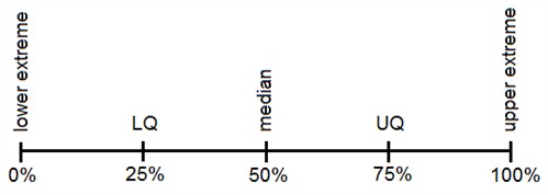
The LQ corresponds to 25% of your data, the median corresponds to 50% of the data and the UQ corresponds to 75% of the data.
The difference between the lower quartile and the upper quartile is called the interquartile range and corresponds to the 50% of the data points that are in the middle
Example
35, 35, 37, 40, 43, 56, 58, 58, 60
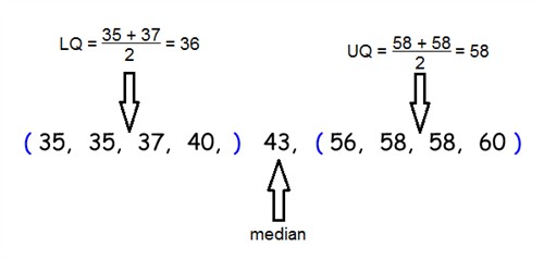
The interquartile range is 58 - 36 = 22
You can use a steam-and-leaf plot to find and display the median, the LQ and the UQ. Here is the stem-and-leaf plot that we made earlier in this section
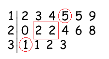
The median is at (22 + 22)/2 = 22 and is marked by a box. The LQ and UQ are marked by circles. The LQ is 15 while the UQ is 31.
It's hard to get a visualized measure of the variation when using the stem-and-leaf plot. Now we're going to introduce a second kind of plot namely the box-and-whiskers plot.
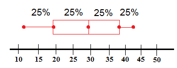
The box-and-whiskers plot is drawn on a number line. It includes a box whose sides are at the LQ and the UQ with a line drawn somewhere in the middle corresponding to the median. From the box two whiskers are drawn. The endpoints of the whiskers are the upper and lower extremes.
To draw a box-and-whiskers plot begin by marking all the above mentioned values.
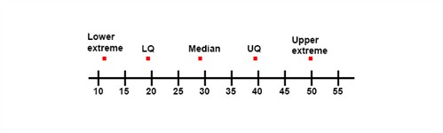
The next step is to draw the box. The box has its sides at the LQ and the UQ and we display the median by drawing a line. Then we extend the whiskers from each quartile to the upper and lower extremes. This box-and-whiskers plot separates the data into quarters; with the same number of data points in each par. The length of the plot corresponds to the measure of variation of the data set. The smaller it is the less is the variation.
Video lesson
Draw a stem-and-leaf plot